When using laser Doppler velocimetry (LDV), the bandpass filter and the downmix frequency within the signal processor should be set appropriately in order to both adequately capture the signal of interest as well as to achieve the best resolution.
To this end, the final goal is to have the narrowest Band Pass filter possible for your flow. This helps us to take full advantage of the resolution of the processor.
Imagine you were tasked with measuring the diameter of a human hair; you wouldn’t use a yardstick! You would use something with much finer demarcations, like a micrometer.
Now, say you have to measure the length of your front yard, you certainly wouldn’t use a micrometer!
Likewise, you could use the widest (50-100MHz) Band Pass for all of your flows, but you would be much better off using a Band Pass that is more suited to your flow, for the highest resolution possible, and also to eliminate ‘noise.’
To do this, it often works well to start out with some nominal values for Band Pass Filter (BPF) and Downmix (DM). Usually, 1-10 MHz is recommended for BPF and 36 is recommended for DM. These values tend to work well for many flows.
Then, take some data. How “wide” is your data in the frequency histogram?
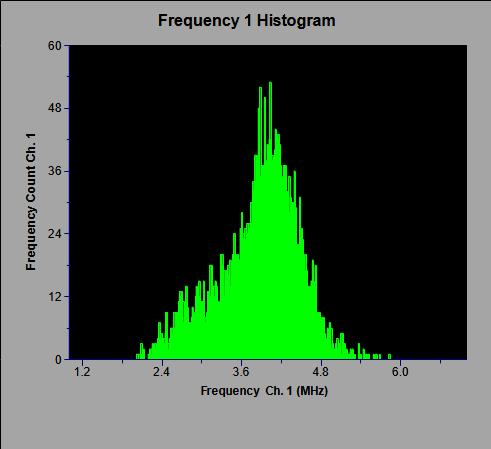
In the case above, the width of the data is from about 2 MHz to 6 MHz, or 4 MHz. So, we want to choose the narrowest BPF that will be able to “hold” this data.

In this case, the narrowest BPF we can use is 1-10 MHz, since the next smallest, 0.3-3 MHz, only has a span of 2.7 MHz.
Once the BPF has been chosen, we want to adjust the DM so that the data peak in the frequency histogram is centered within the BPF, or near the lower end of the BPF, without “clipping” data. This allows us to maximize the resolution within our BPF.
Below is an example of some data that appears “clipped” near 1 MHz:
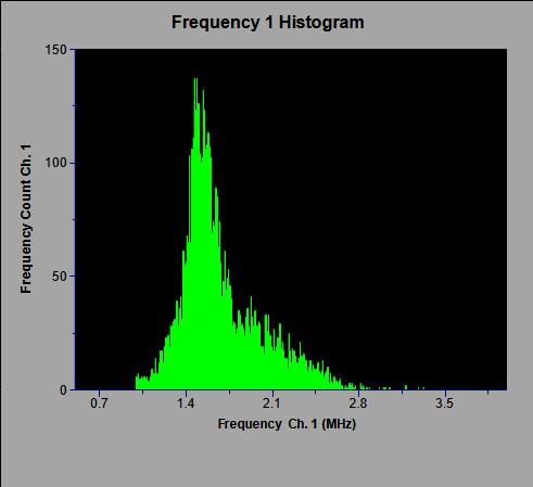
In this case, we would want to lower the DM so that no data is clipped.
(Note: Lowering the DM value has the effect of shifting the data toward higher frequencies.)
Your BPF and DM settings are now optimized.
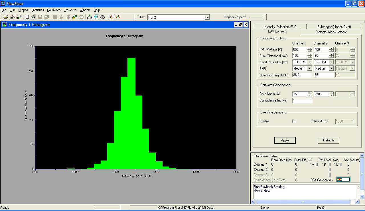
Here is another example:

Note that the ‘width’ of the frequencies measured goes from about 1.44 to 1.56, a width of about 0.12 MHz. For this we could go down to 0.1 – 1 MHz, or maybe even 30 – 300 KHz, as long as we adjust the DM appropriately.
However, for this experiment, the user is expecting to have some variation from these values, and doesn’t want to go to that narrow BPF, in case there are velocities (frequencies) slightly outside this range for some of the datasets. For this reason, the bandpass was narrowed from 1-10 MHz, down to 0.3 – 3MHz. Then the downmix had to be adjusted from 36 MHz to 38.5 MHz. to get the data centered on this new frequency band.
